Importing and manipulating data for TRANSPIRE analysis¶

The backbone of analysis with TRANSPIRE relies heavily on Pandas DataFrames with multi-level indicies. This provides a powerful and flexible framework for data manipulation. To make this analysis more accessible to those without a strong background or familiarity with Pandas, TRANSPIRE provides utilities to simplify data loading and manipulation. For more advanced users, they may prefer to forego the built-in TRANSPIRE utilities for their own functions.

[47]:

import TRANSPIRE

1. Define file path and load data¶

[48]:

f = 'mydata_no_localizations.csv'
df = TRANSPIRE.data.import_data.load_data(f)

df

[48]:

	condition	uninfected						infected
	fraction	1	2	3	4	5	6	1	2	3	4	5	6
accession	gene name
A0AVT1	UBA6	0.342416	0.346408	0.147271	0.090486	0.043105	0.030314	0.056764	0.095989	0.094597	0.139616	0.345400	0.257444
A0FGR8	ESYT2	0.200266	0.288014	0.264795	0.152079	0.061482	0.020638	0.141740	0.250193	0.250726	0.142513	0.153470	0.049585
A1L0T0	ILVBL	0.193194	0.333657	0.239388	0.160094	0.065503	0.018098	0.127224	0.265472	0.228027	0.143158	0.173794	0.054383
A1L188	NDUFAF8	NaN	NaN	NaN	NaN	NaN	NaN	0.034472	0.063834	0.198874	0.395500	0.214612	0.092709
A2RRP1	NBAS	0.266384	0.305499	0.207475	0.134155	0.052810	0.019836	0.155677	0.248836	0.210393	0.128968	0.163133	0.082520
...	...	...	...	...	...	...	...	...	...	...	...	...	...
Q9Y6Q2	STON1	0.468515	0.291495	0.107717	0.079150	0.037682	0.015441	NaN	NaN	NaN	NaN	NaN	NaN
Q9Y6R0	NUMBL	0.281558	0.325676	0.221316	0.099426	0.049386	0.022638	NaN	NaN	NaN	NaN	NaN	NaN
Q9Y6R1	SLC4A4	0.319321	0.299931	0.208633	0.104363	0.042091	0.017095	NaN	NaN	NaN	NaN	NaN	NaN
Q9Y6V0	PCLO	0.289078	0.369018	0.110457	0.088003	0.097068	0.014004	0.204732	0.314821	0.167343	0.128688	0.131086	0.053329
Q9Y6W5	WASF2	0.483214	0.298740	0.120254	0.054733	0.034164	0.014242	NaN	NaN	NaN	NaN	NaN	NaN

3304 rows × 12 columns

Note that the DataFrame above does not contain a “localization” index level. Thus, we need to assign a set of organelle markers to the data in order to run the TRANSPIRE analysis.

2. Add subcellular localization annotation to markers (optional)¶

[49]:

df_with_markers = TRANSPIRE.data.import_data.add_markers(df, 'human_fibroblast')

df_with_markers

[49]:

		condition	uninfected						infected
		fraction	1	2	3	4	5	6	1	2	3	4	5	6
accession	gene name	localization
A0AVT1	UBA6	NaN	0.342416	0.346408	0.147271	0.090486	0.043105	0.030314	0.056764	0.095989	0.094597	0.139616	0.345400	0.257444
A0FGR8	ESYT2	NaN	0.200266	0.288014	0.264795	0.152079	0.061482	0.020638	0.141740	0.250193	0.250726	0.142513	0.153470	0.049585
A1L0T0	ILVBL	NaN	0.193194	0.333657	0.239388	0.160094	0.065503	0.018098	0.127224	0.265472	0.228027	0.143158	0.173794	0.054383
A1L188	NDUFAF8	NaN	NaN	NaN	NaN	NaN	NaN	NaN	0.034472	0.063834	0.198874	0.395500	0.214612	0.092709
A2RRP1	NBAS	NaN	0.266384	0.305499	0.207475	0.134155	0.052810	0.019836	0.155677	0.248836	0.210393	0.128968	0.163133	0.082520
...	...	...	...	...	...	...	...	...	...	...	...	...	...	...
Q9Y6Q2	STON1	Cytosol	0.468515	0.291495	0.107717	0.079150	0.037682	0.015441	NaN	NaN	NaN	NaN	NaN	NaN
Q9Y6R0	NUMBL	NaN	0.281558	0.325676	0.221316	0.099426	0.049386	0.022638	NaN	NaN	NaN	NaN	NaN	NaN
Q9Y6R1	SLC4A4	NaN	0.319321	0.299931	0.208633	0.104363	0.042091	0.017095	NaN	NaN	NaN	NaN	NaN	NaN
Q9Y6V0	PCLO	NaN	0.289078	0.369018	0.110457	0.088003	0.097068	0.014004	0.204732	0.314821	0.167343	0.128688	0.131086	0.053329
Q9Y6W5	WASF2	Cytosol	0.483214	0.298740	0.120254	0.054733	0.034164	0.014242	NaN	NaN	NaN	NaN	NaN	NaN

3304 rows × 12 columns

Notice how this DataFrame now has a “localization” index level. At this point, we should visualize our data and see how well-separated are organelle marker classes are to determine if we should group any together (e.g. for less-complex fractionation workflows).

[35]:

# select the subset of the dataframe with non-null localization values (i.e. the markers)
marker_profiles = df_with_markers[df_with_markers.index.get_level_values('localization').notnull()]

# pivot the dataframe so that the "condition" column level is now an index level
marker_profiles_pivot = marker_profiles.stack('condition')

# "melt" the dataframe so that the fractions across the top of the dataframe
# become their own column of values, associated with a corresponding relative abundance value
markers_to_plot = marker_profiles_pivot.reset_index().melt(marker_profiles_pivot.index.names)

markers_to_plot

[35]:

	accession	gene name	localization	condition	fraction	value
0	O00115	DNASE2	Lysosome	infected	1	0.091988
1	O00115	DNASE2	Lysosome	uninfected	1	0.121081
2	O00116	AGPS	Peroxisome	infected	1	0.035467
3	O00116	AGPS	Peroxisome	uninfected	1	0.066992
4	O00151	PDLIM1	Cytosol	infected	1	0.298505
...	...	...	...	...	...	...
5743	Q9Y6G9	DYNC1LI1	Cytosol	uninfected	6	0.030355
5744	Q9Y6N5	SQOR	Mitochondria	infected	6	0.127455
5745	Q9Y6N5	SQOR	Mitochondria	uninfected	6	0.049427
5746	Q9Y6Q2	STON1	Cytosol	uninfected	6	0.015441
5747	Q9Y6W5	WASF2	Cytosol	uninfected	6	0.014242

5748 rows × 6 columns

*Now, lets look at the marker protein profiles*

[36]:

import seaborn as sns
import matplotlib.pyplot as plt

g = sns.FacetGrid(data = markers_to_plot, col = 'condition', hue='localization')
g.map(sns.lineplot, 'fraction','value')
g.add_legend()
plt.show()

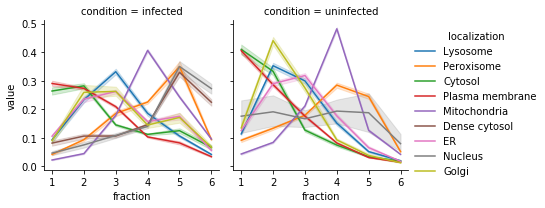
../_images/notebooks_importing_and_manipulating_data_11_0.png

In this data, we can see that the plasma membrane and cytosol have overlapping profiles. Same with the ER, Lysosome, and Golgi, as well as the Dense cytosol and nucleus. If we desire, TRANSPIRE has a built in utility to group organlles together. Note that organelles excluded from the mapping defined below will retain their original assignments

[51]:

organelle_mapping = {

    'ER': 'ER/Golgi/Lysosome',
    'Golgi': 'ER/Golgi/Lysosome',
    'Lysosome': 'ER/Golgi/Lysosome',
    'Plasma membrane':'PM/Cytosol',
    'Cytosol': 'PM/Cytosol',
    'Dense cytosol': 'DC/Nucleus',
    'Nucleus': 'DC/Nucleus'

}

df_grouped = TRANSPIRE.utils.group_organelles(df_with_markers, organelle_mapping)

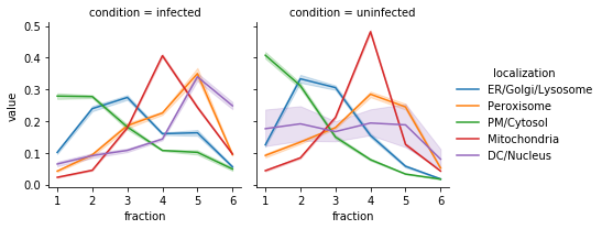
Now if we plot the profiles of the grouped markers, we can see that they are much more clearly separated¶

[38]:

g = sns.FacetGrid(data = df_grouped.stack('condition').reset_index().melt(df_grouped.index.names+['condition']),
                  col = 'condition', hue='localization')
g.map(sns.lineplot, 'fraction','value')
g.add_legend()
plt.show()

../_images/notebooks_importing_and_manipulating_data_15_0.png

3. Define comparisons to make¶

Now we need to define which conditions we want to make comparisons between. In this dataset, we only have infected vs. uninfected conditions. Note that these comparisons MUST match the names of your condition columns–otherwise TRANSPIRE will fail

[39]:

comparisons = [('uninfected', 'infected')]

4. Generate synthetic translocations and label encodings¶

[41]:

synthetic_translocations = TRANSPIRE.data.generate_translocations.make_translocations(df_grouped, comparisons)

synthetic_translocations

[41]:

									1	2	3	4	5	6	7	8	9	10	11	12
accession_A	gene name_A	localization_A	condition_A	accession_B	gene name_B	localization_B	condition_B	label
O00115	DNASE2	ER/Golgi/Lysosome	uninfected	O00115	DNASE2	ER/Golgi/Lysosome	infected	ER/Golgi/Lysosome to ER/Golgi/Lysosome	0.121081	0.378059	0.287889	0.142575	0.056295	0.014235	0.091988	0.249011	0.334238	0.181254	0.104927	0.041090
				O00116	AGPS	Peroxisome	infected	ER/Golgi/Lysosome to Peroxisome	0.121081	0.378059	0.287889	0.142575	0.056295	0.014235	0.035467	0.087956	0.190615	0.228672	0.353767	0.095804
				O00151	PDLIM1	PM/Cytosol	infected	ER/Golgi/Lysosome to PM/Cytosol	0.121081	0.378059	0.287889	0.142575	0.056295	0.014235	0.298505	0.273591	0.136350	0.124446	0.101276	0.051836
				O00161	SNAP23	PM/Cytosol	infected	ER/Golgi/Lysosome to PM/Cytosol	0.121081	0.378059	0.287889	0.142575	0.056295	0.014235	0.303401	0.275456	0.219409	0.094259	0.065571	0.027320
				O00186	STXBP3	PM/Cytosol	infected	ER/Golgi/Lysosome to PM/Cytosol	0.121081	0.378059	0.287889	0.142575	0.056295	0.014235	0.251250	0.279922	0.220812	0.102742	0.089897	0.047200
...	...	...	...	...	...	...	...	...	...	...	...	...	...	...	...	...	...	...	...	...
Q9Y6N5	SQOR	Mitochondria	uninfected	Q9Y673	ALG5	ER/Golgi/Lysosome	infected	Mitochondria to ER/Golgi/Lysosome	0.035159	0.085702	0.215704	0.471670	0.115302	0.049427	0.141876	0.246472	0.287558	0.145362	0.118529	0.041669
				Q9Y676	MRPS18B	Mitochondria	infected	Mitochondria to Mitochondria	0.035159	0.085702	0.215704	0.471670	0.115302	0.049427	0.016078	0.036276	0.165740	0.417482	0.257843	0.093664
				Q9Y680	FKBP7	ER/Golgi/Lysosome	infected	Mitochondria to ER/Golgi/Lysosome	0.035159	0.085702	0.215704	0.471670	0.115302	0.049427	0.129000	0.285763	0.290694	0.140269	0.108666	0.037075
				Q9Y6G3	MRPL42	Mitochondria	infected	Mitochondria to Mitochondria	0.035159	0.085702	0.215704	0.471670	0.115302	0.049427	0.022533	0.052818	0.178052	0.399956	0.237964	0.098262
				Q9Y6N5	SQOR	Mitochondria	infected	Mitochondria to Mitochondria	0.035159	0.085702	0.215704	0.471670	0.115302	0.049427	0.023746	0.042218	0.201027	0.353196	0.246338	0.127455

147456 rows × 12 columns

[44]:

# generate mappings to encode the labels as integers for model training
mapping, mapping_r = TRANSPIRE.utils.get_mapping(df_grouped)

mapping # for encoding labels

[44]:

DC/Nucleus to DC/Nucleus                   0
DC/Nucleus to ER/Golgi/Lysosome            1
DC/Nucleus to Mitochondria                 2
DC/Nucleus to PM/Cytosol                   3
DC/Nucleus to Peroxisome                   4
ER/Golgi/Lysosome to DC/Nucleus            5
ER/Golgi/Lysosome to ER/Golgi/Lysosome     6
ER/Golgi/Lysosome to Mitochondria          7
ER/Golgi/Lysosome to PM/Cytosol            8
ER/Golgi/Lysosome to Peroxisome            9
Mitochondria to DC/Nucleus                10
Mitochondria to ER/Golgi/Lysosome         11
Mitochondria to Mitochondria              12
Mitochondria to PM/Cytosol                13
Mitochondria to Peroxisome                14
PM/Cytosol to DC/Nucleus                  15
PM/Cytosol to ER/Golgi/Lysosome           16
PM/Cytosol to Mitochondria                17
PM/Cytosol to PM/Cytosol                  18
PM/Cytosol to Peroxisome                  19
Peroxisome to DC/Nucleus                  20
Peroxisome to ER/Golgi/Lysosome           21
Peroxisome to Mitochondria                22
Peroxisome to PM/Cytosol                  23
Peroxisome to Peroxisome                  24
dtype: int64

[45]:

mapping_r # for de-encoding labels

[45]:

0                   DC/Nucleus to DC/Nucleus
1            DC/Nucleus to ER/Golgi/Lysosome
2                 DC/Nucleus to Mitochondria
3                   DC/Nucleus to PM/Cytosol
4                   DC/Nucleus to Peroxisome
5            ER/Golgi/Lysosome to DC/Nucleus
6     ER/Golgi/Lysosome to ER/Golgi/Lysosome
7          ER/Golgi/Lysosome to Mitochondria
8            ER/Golgi/Lysosome to PM/Cytosol
9            ER/Golgi/Lysosome to Peroxisome
10                Mitochondria to DC/Nucleus
11         Mitochondria to ER/Golgi/Lysosome
12              Mitochondria to Mitochondria
13                Mitochondria to PM/Cytosol
14                Mitochondria to Peroxisome
15                  PM/Cytosol to DC/Nucleus
16           PM/Cytosol to ER/Golgi/Lysosome
17                PM/Cytosol to Mitochondria
18                  PM/Cytosol to PM/Cytosol
19                  PM/Cytosol to Peroxisome
20                  Peroxisome to DC/Nucleus
21           Peroxisome to ER/Golgi/Lysosome
22                Peroxisome to Mitochondria
23                  Peroxisome to PM/Cytosol
24                  Peroxisome to Peroxisome
dtype: object

Now we have generated the synthetic translocation profiles that TRANSPIRE requires for model training and analysis. See the next notebook on hyperparameter optimization or skip to the notebook on final model fitting and evaluation to learn how to build and fit models for subsequent analysis